A Tale of Two Hawks Part 2

A reproducible analysis of college basketball data with R

Introduction

For context, please see Part 1 here.

What We’re Looking For

If the goal is to use data to bet responsible AND share our results in reproducible manner, we need to isolate the data that helps us develop a model that predicts winners in potential match-ups.

Dean Oliver narrowed the most important analytics of college basketball down to Four Factors:

1. Shooting Efficiency - More baskets and fewer misses
2. Turnovers - Number of times losing a possession
3. Rebounds - Number of times gaining a possession
4. Free Throws - Free points

Additionally, there are efficiency ratings - points scored and allowed per 100 possessions - which help adjust for pace.

When we talk about using machine learning to help us predict the outcome of match-ups, what we are actually doing is identifying features of a phenomena that could potentially assist us in determining outcomes. That is incredibly boiled down, but when we develop these predictive models, the models themselves let the analysts know what features are driving most of the explanation.

---

How You Can Use This

We are going to take a look at a hypothetical match-up between the Kansas Jayhawks and the Miami RedHawks. There is a slight chance they could in fact end up playing each other in the tournament IF they are in the same region. There is likely no chance they both make it to the Final Four.

This exact workflow works for any team in Division I basketball.

The steps:

1. Load schedule and box scores with hoopR
2. Calculate four factors using the formulas above
3. Calculate efficiency ratings
4. Visualize trends with ggplot2
5. Compare head-to-head results

---

Step 1: Retrieve official ESPN data

Loading data using the help of an R package named hoopR. You can learn more about its documentation, but it’s basically an API call to EPSN for live college basketball data.

I am using other libraries of course, but we don’t have time to talk about them!

Code

library(ggplot2)
library(dplyr)

Attaching package: 'dplyr'

The following objects are masked from 'package:stats':

    filter, lag

The following objects are masked from 'package:base':

    intersect, setdiff, setequal, union

Code

library(hoopR)

Warning: package 'hoopR' was built under R version 4.5.2

Code

library(janitor)

Warning: package 'janitor' was built under R version 4.5.2

Attaching package: 'janitor'

The following objects are masked from 'package:stats':

    chisq.test, fisher.test

Code

schedule <- 
  load_mbb_schedule(seasons = 2026) |>
  clean_names()

box_scores <- 
  load_mbb_team_box(seasons = 2026) |>
  clean_names()

# Filter to just Kansas & Miami
hawks <- 
  box_scores |>
  filter(team_display_name %in% c("Kansas Jayhawks", "Miami (OH) RedHawks"))

# Quick look at what we have
str(hawks[1:2,])

hoopR_dt [2 × 59] (S3: hoopR_data/tbl_df/tbl/data.table/data.frame)
 $ game_id                          : int [1:2] 401827690 401814572
 $ season                           : int [1:2] 2026 2026
 $ season_type                      : int [1:2] 2 2
 $ game_date                        : Date[1:2], format: "2026-02-18" "2026-02-17"
 $ game_date_time                   : POSIXct[1:2], format: "2026-02-18 21:00:00" "2026-02-17 19:00:00"
 $ team_id                          : int [1:2] 2305 193
 $ team_uid                         : chr [1:2] "s:40~l:41~t:2305" "s:40~l:41~t:193"
 $ team_slug                        : chr [1:2] "kansas-jayhawks" "miami-oh-redhawks"
 $ team_location                    : chr [1:2] "Kansas" "Miami (OH)"
 $ team_name                        : chr [1:2] "Jayhawks" "RedHawks"
 $ team_abbreviation                : chr [1:2] "KU" "M-OH"
 $ team_display_name                : chr [1:2] "Kansas Jayhawks" "Miami (OH) RedHawks"
 $ team_short_display_name          : chr [1:2] "Kansas" "Miami OH"
 $ team_color                       : chr [1:2] "0051ba" "c41230"
 $ team_alternate_color             : chr [1:2] "e8000d" "ffffff"
 $ team_logo                        : chr [1:2] "https://a.espncdn.com/i/teamlogos/ncaa/500/2305.png" "https://a.espncdn.com/i/teamlogos/ncaa/500/193.png"
 $ team_home_away                   : chr [1:2] "away" "away"
 $ team_score                       : int [1:2] 81 86
 $ team_winner                      : logi [1:2] TRUE TRUE
 $ assists                          : int [1:2] 20 16
 $ blocks                           : int [1:2] 7 1
 $ defensive_rebounds               : int [1:2] 31 22
 $ fast_break_points                : chr [1:2] "10" "9"
 $ field_goal_pct                   : num [1:2] 46 50
 $ field_goals_made                 : int [1:2] 28 26
 $ field_goals_attempted            : int [1:2] 61 52
 $ flagrant_fouls                   : int [1:2] 0 0
 $ fouls                            : int [1:2] 14 15
 $ free_throw_pct                   : num [1:2] 88 73
 $ free_throws_made                 : int [1:2] 14 24
 $ free_throws_attempted            : int [1:2] 16 33
 $ largest_lead                     : chr [1:2] "23" "10"
 $ lead_changes                     : chr [1:2] "0" "2"
 $ lead_percentage                  : chr [1:2] "99" "91"
 $ offensive_rebounds               : int [1:2] 10 4
 $ points_in_paint                  : chr [1:2] "32" "28"
 $ steals                           : int [1:2] 5 9
 $ team_turnovers                   : int [1:2] 0 1
 $ technical_fouls                  : int [1:2] 0 0
 $ three_point_field_goal_pct       : num [1:2] 46 43
 $ three_point_field_goals_made     : int [1:2] 11 10
 $ three_point_field_goals_attempted: int [1:2] 24 23
 $ total_rebounds                   : int [1:2] 41 26
 $ total_technical_fouls            : int [1:2] 0 0
 $ total_turnovers                  : int [1:2] 12 7
 $ turnover_points                  : chr [1:2] "11" "14"
 $ turnovers                        : int [1:2] 12 7
 $ opponent_team_id                 : int [1:2] 197 113
 $ opponent_team_uid                : chr [1:2] "s:40~l:41~t:197" "s:40~l:41~t:113"
 $ opponent_team_slug               : chr [1:2] "oklahoma-state-cowboys" "massachusetts-minutemen"
 $ opponent_team_location           : chr [1:2] "Oklahoma State" "Massachusetts"
 $ opponent_team_name               : chr [1:2] "Cowboys" "Minutemen"
 $ opponent_team_abbreviation       : chr [1:2] "OKST" "MASS"
 $ opponent_team_display_name       : chr [1:2] "Oklahoma State Cowboys" "Massachusetts Minutemen"
 $ opponent_team_short_display_name : chr [1:2] "Oklahoma St" "UMass"
 $ opponent_team_color              : chr [1:2] "fe5c00" "881c1c"
 $ opponent_team_alternate_color    : chr [1:2] "000000" "ffffff"
 $ opponent_team_logo               : chr [1:2] "https://a.espncdn.com/i/teamlogos/ncaa/500/197.png" "https://a.espncdn.com/i/teamlogos/ncaa/500/113.png"
 $ opponent_team_score              : int [1:2] 69 77
 - attr(*, "hoopR_timestamp")= POSIXct[1:1], format: "2026-02-19 08:00:53"
 - attr(*, "hoopR_type")= chr "ESPN MBB Team Boxscores from hoopR data repository"

I’ve taken the first two rows of our hawks data frame, which was filtered from the 2026 box score data stored in box_scores and told R to give me its structure. We have 59 columns; R lists them in order of appearance in the matrix, defines the type of data we are dealing with, shows us how many observations and then gives us a preview of said observations.

We can see that these are the most recent games for both teams.

---

Step 2: Calculate the Four Factors

Now let’s calculate Oliver’s Four Factors for both teams.

Code

four_factors <- 
  hawks |>
  mutate(
    # Effective Field Goal % (weights three-pointers appropriately)
    efg_pct = (field_goals_made + 0.5 * three_point_field_goals_made) / 
              field_goals_attempted,
    
    # Turnover % (turnovers per 100 possessions)
    tov_pct = turnovers / 
              (field_goals_attempted + 0.44 * free_throws_attempted + turnovers),
    
    # Offensive Rebound % (offensive rebounds captured)
    orb_pct = offensive_rebounds / 
              (offensive_rebounds + defensive_rebounds),
    
    # Free Throw Rate (free throw attempts per field goal attempt)
    ft_rate = free_throws_made / field_goals_attempted
  ) |>
  select(team_display_name, game_date, team_score, opponent_team_score,
         efg_pct, tov_pct, orb_pct, ft_rate)

# Show the first few games
head(four_factors, 10) |> knitr::kable()

team_display_name	game_date	team_score	opponent_team_score	efg_pct	tov_pct	orb_pct	ft_rate
Kansas Jayhawks	2026-02-18	81	69	0.5491803	0.1499250	0.2439024	0.2295082
Miami (OH) RedHawks	2026-02-17	86	77	0.5961538	0.0952122	0.1538462	0.4615385
Kansas Jayhawks	2026-02-14	56	74	0.4313725	0.1841360	0.2941176	0.2352941
Miami (OH) RedHawks	2026-02-13	90	74	0.5948276	0.1134644	0.2105263	0.3620690
Kansas Jayhawks	2026-02-09	82	78	0.4420290	0.1208791	0.4146341	0.3043478
Miami (OH) RedHawks	2026-02-07	90	74	0.6271186	0.1600197	0.3000000	0.2711864
Kansas Jayhawks	2026-02-07	71	59	0.5267857	0.1369113	0.1944444	0.2142857
Miami (OH) RedHawks	2026-02-03	73	71	0.6034483	0.1765345	0.1785714	0.0517241
Kansas Jayhawks	2026-02-02	64	61	0.5094340	0.2034726	0.1315789	0.1886792
Kansas Jayhawks	2026-01-31	90	82	0.6696429	0.0826902	0.1250000	0.2678571

---

Step 3: Compare Season Averages

Let’s see which team has the edge in each factor.

Code

season_averages <- 
  four_factors |>
  group_by(team_display_name) |>
  summarise(
    games = n(),
    avg_efg = mean(efg_pct, na.rm = TRUE),
    avg_tov = mean(tov_pct, na.rm = TRUE),
    avg_orb = mean(orb_pct, na.rm = TRUE),
    avg_ftr = mean(ft_rate, na.rm = TRUE),
    .groups = "drop"
  )

library(kableExtra)

Warning: package 'kableExtra' was built under R version 4.5.2

Attaching package: 'kableExtra'

The following object is masked from 'package:dplyr':

    group_rows

Code

season_averages |>
  knitr::kable(
    digits = 3,
    col.names = c("Team", "Games", "eFG%", "TOV%", "ORB%", "FTR"),
    caption = "Season Averages: Four Factors",
    format = "html",
    escape = FALSE
  ) |>
  kable_styling(bootstrap_options = c("striped", "hover")) |>
  # Highlight max eFG% (higher is better)
  column_spec(3, 
              background = ifelse(season_averages$avg_efg == max(season_averages$avg_efg),
                                  "#d4edda", "white")) |>
  # Highlight min TOV% (lower is better)  
  column_spec(4,
              background = ifelse(season_averages$avg_tov == min(season_averages$avg_tov),
                                  "#d4edda", "white")) |>
  # Highlight max ORB% (higher is better)
  column_spec(5,
              background = ifelse(season_averages$avg_orb == max(season_averages$avg_orb),
                                  "#d4edda", "white")) |>
  # Highlight max FTR (higher is better)
  column_spec(6,
              background = ifelse(season_averages$avg_ftr == max(season_averages$avg_ftr),
                                  "#d4edda", "white"))

Season Averages: Four Factors

Team	Games	eFG%	TOV%	ORB%	FTR
Kansas Jayhawks	26	0.535	0.136	0.244	0.259
Miami (OH) RedHawks	26	0.621	0.133	0.225	0.312

---

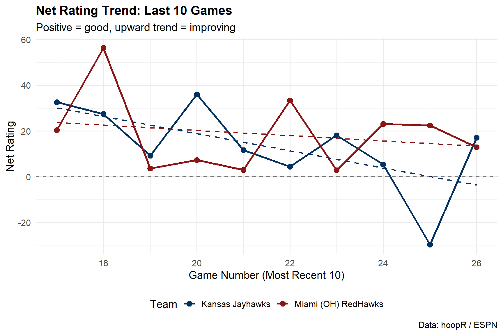
Would you look at that. Miami’s offense outperforms Kansas…if you completely ignore the quality of opponents Miami has played vs Kansas. The Big 12 has Houston, Arizona, Iowa State, Texas Tech and BYU in the AP Top 25 along with Kansas. Miami’s best win as a 3-point home win over Akron.

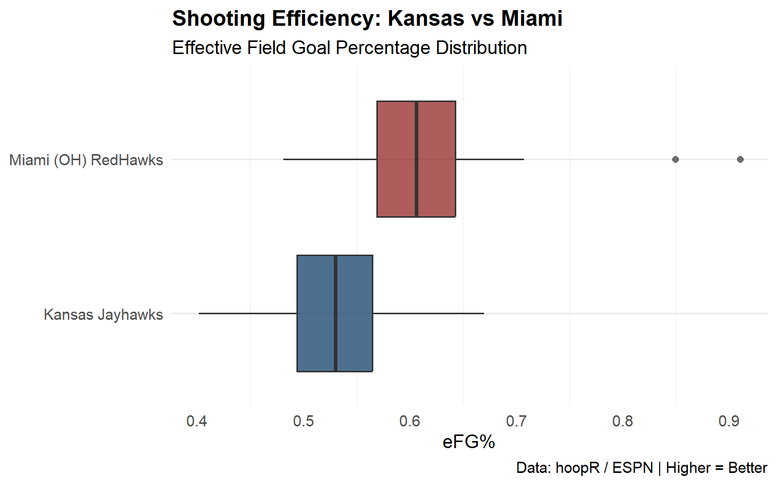
Step 4: Visualize Shooting Efficiency

Let’s look at how consistent each team is at making shots.

Code

four_factors |>
  ggplot(aes(x = team_display_name, y = efg_pct, fill = team_display_name)) +
  geom_boxplot(alpha = 0.7, show.legend = FALSE) +
  scale_fill_manual(
    values = c("Kansas Jayhawks" = "#003262", 
               "Miami (OH) RedHawks" = "#8C1515")
  ) +
  labs(
    title = "Shooting Efficiency: Kansas vs Miami",
    subtitle = "Effective Field Goal Percentage Distribution",
    x = NULL,
    y = "eFG%",
    caption = "Data: hoopR / ESPN | Higher = Better"
  ) +
  theme_minimal(base_size = 14) +
  theme(
    plot.title = element_text(face = "bold", size = 16),
    panel.grid.major.x = element_blank()
  ) +
  coord_flip()

It’s very likely Kansas is playing teams with much, much better defenses.

Step 5: Calculate Efficiency Ratings

Points per game is misleading because it depends on pace. A team that plays fast will score more points, but that doesn’t mean they’re better.

Efficiency ratings adjust for pace by measuring points per 100 possessions.

Code

efficiency <- hawks %>%
  mutate(
    # Estimate possessions using the standard formula
    possessions = field_goals_attempted - 
                  offensive_rebounds + 
                  turnovers + 
                  0.44 * free_throws_attempted,
    
    # Offensive Rating (points scored per 100 possessions)
    ortg = (team_score / possessions) * 100,
    
    # Defensive Rating (points allowed per 100 possessions)
    drtg = (opponent_team_score / possessions) * 100,
    
    # Net Rating (offense minus defense)
    net_rating = ortg - drtg
  ) %>%
  select(team_display_name, game_date, possessions, ortg, drtg, net_rating)

# Season averages
efficiency_summary <- efficiency %>%
  group_by(team_display_name) %>%
  summarise(
    avg_pace = mean(possessions, na.rm = TRUE),
    avg_ortg = mean(ortg, na.rm = TRUE),
    avg_drtg = mean(drtg, na.rm = TRUE),
    avg_net = mean(net_rating, na.rm = TRUE),
    .groups = "drop"
  )

efficiency_summary %>%
  knitr::kable(
    digits = 1,
    col.names = c("Team", "Pace", "ORtg", "DRtg", "Net Rating"),
    caption = "Efficiency Ratings (per 100 possessions)"
  )

Efficiency Ratings (per 100 possessions)

Team	Pace	ORtg	DRtg	Net Rating
Kansas Jayhawks	67.9	113.8	100.1	13.7
Miami (OH) RedHawks	72.4	127.0	102.7	24.3

Offensive Rating (ORtg): Points per 100 possessions

Defensive Rating (DRtg): Points allowed per 100 possessions

Net Rating: Offensive Rating minus Defensive Rating

Step 6: Recent Form (Last 10 Games)

Let’s see who’s trending up and who’s trending down.

Code

efficiency %>%
  group_by(team_display_name) %>%
  arrange(game_date) %>%
  mutate(game_num = row_number()) %>%
  filter(game_num > max(game_num) - 10) %>%
  ggplot(aes(x = game_num, y = net_rating, color = team_display_name)) +
  geom_line(linewidth = 1.2) +
  geom_point(size = 3) +
  geom_hline(yintercept = 0, linetype = "dashed", color = "gray50") +
  geom_smooth(method = "lm", se = FALSE, linetype = "dashed", linewidth = 0.8) +
  scale_color_manual(
    values = c("Kansas Jayhawks" = "#003262", 
               "Miami (OH) RedHawks" = "#8C1515")
  ) +
  labs(
    title = "Net Rating Trend: Last 10 Games",
    subtitle = "Positive = good, upward trend = improving",
    x = "Game Number (Most Recent 10)",
    y = "Net Rating",
    color = "Team",
    caption = "Data: hoopR / ESPN"
  ) +
  theme_minimal(base_size = 14) +
  theme(
    plot.title = element_text(face = "bold", size = 16),
    legend.position = "bottom"
  )

`geom_smooth()` using formula = 'y ~ x'

Miami appears to be in a more stable position than Kansas. As a unit, Miami definitely seems more consistent.

Conclusion

This workflow can be reproduced for any of the 360+ Division-1 Mens’ Basketball Teams. In Part 3 of this series, we’ll walk through how to build machine learning models to incorporate all of this data and predict who would win in a potential match-up between Kansas and Miami, the margin of victory and the total points scored.

Want to see more analyses like this? Subscribe to our Telegram for daily picks and breakdowns.